You are truly growing your Excel skills, it seems. That is the primary reason why you are visiting this page – since “With Excel usage comes data…with data comes pairs at times triplicate data…”. You, too, are stuck right now in this mesh of duplicates and triplicates – which is why a new tab on your monitor gives way to a page that answers the question – how to find duplicates in Excel?
As you will scroll down this write-up, you will find a detailed process of finding matching pairs in workbook spreadsheet and removing them or using them accordingly. Hopefully, you will be able to comprehend the process and act accordingly. Please proceed.
Table of Contents
How to find duplicates in Excel?
There are multiple formulas that you can use to find the matching pairs in the sheet. They are –
1. The Conditional Formatting –
This feature is available in the Styles section of the sheet, where you will have to choose Highlight Cell Rules and the Duplicate Value. As you follow these steps, immediately, a pop-up window will depict the matching pairs’ values, and you will be able to filter them. The filtering of the matching pair data is most important since, once you are done doing that – you can automatically remove them accordingly.
This feature is available in all the Excel versions post-2007 and is surely one of the most convenient modes to deal with the corresponding data.

2. The Specific Occurrence in terms of Conditional Formatting –
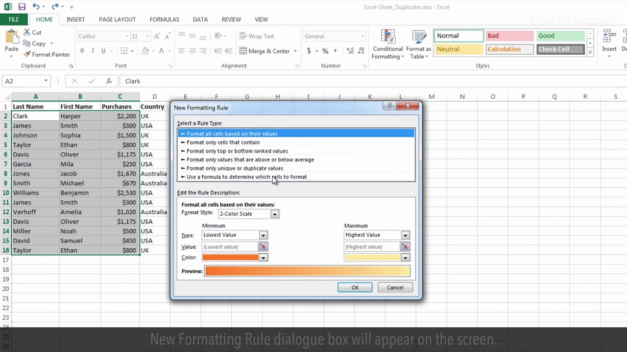
What would you do if you had to figure out the number of times this duplicity of values has happened? In that case – there is the usage of the COUNTIF formula. In this case, there is the New Formatting Rule that helps you select the type of the rule and do the required editing.
The main function of the COUNTIF formula is to highlight those duplicate cells with triplicate or multiple counts.
The data range used in this case is A2:C8.
3. Removing Duplicates using the spreadsheet of the workbook itself
When searching for a matching pair in the Excel sheet, at times, you will need to implement old formulas removing the given ones. For that, you will have to enable the Clear Rules icon and then either select the cells from where data has to be removed, or you can remove it from the whole sheet. Now, automatically as you are in the process – you will notice that there are matching pairs (they will have to be highlighted). The next step is to remove them.
#Just a piece of advice – Do keep a copy of the corresponding data since this will be completely deleted.
4. The COUNTIF process
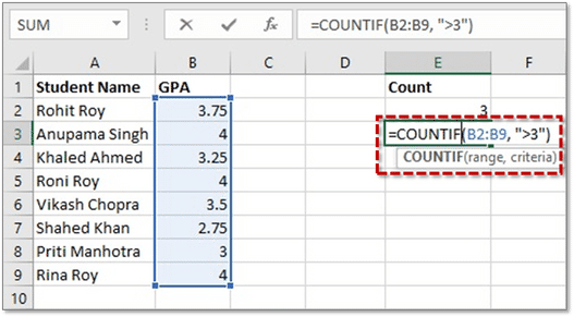
This is surely the most used process – wherein that column that actually has the duplicate entries returns the number of the parallel matching pair for every cell. As you put in the formula (mentioned below) – you will have to pull the formula till the table end and after that, fill up the B2 cell that will be given. It is in the following image that you will get to see the output of the formula.
# Would you like to know the COUNTIF formula?
It is – COUNTIF (A: A, A2)>1 (taking into account that the topmost starter cell is A2)
The data range used in this case is B2:B9.

How to prevent the entry of duplicate data into Workbook?
As you have seen in the above-mentioned portion, the answer to how to find duplicates in Excel has been given. However, it is better to be safe than sorry. So, how would you prevent this entry of corresponding similar data in workbook sheets?
Here are some of the techniques to follow –
Firstly, you will always have to select the range of cells where you wish to prevent the matching pair value. Now go ahead and choose Validation from the Data menu. From here, you will have to Customise, enter the COUNTIF formula and try entering the Duplicate Entry. Immediately – when you try entering a duplicate value, the Excel sheet will reject it, and then you can enter the valid value.
What if you have to deal with triplicates?
Mostly, the issues in Workbook are associated with the corresponding data. However, at times – due to certain incongruencies, data gets repeated three times. What do you do then? The steps are similar to that of in duplicate issue, just that here you will have to use the COUNTIF formula in a detailed manner. It can get a bit dicey – but nothing much to worry about. Also, remember that the formulas that are used in Workbook are cell-based; hence – you can clearly find out which specific cell is being used.

The Styles section of Workbook has the Conditional Formatting icon – you will have to go back there after you choose the range of your cell. Now, you will find that below the button of Icon Sets, there’s a New Rule formula – that provides the menu for the new rules. The next query that the Workbook sheet will put before you is – which of the cells require formatting – to which you will have to click on the icon that states – Use a formula to determine which cells to format. Now place the COUNTIF formula and enter the amount of 3 (triplicate issue). This will target the required rows of 3’s and solve the issue accordingly.
You must note that matching pair data is not invalid in the Workbook sheet, but while one tallies the results, there is a discrepancy. Hence, from next time onwards, please be very careful with the entries. Hopefully, this article on finding duplicates in Excel will help solve the current problem you are facing.

